Methods for use with discovery and replication GWASs
discovery_replication.RmdOur R package, winnerscurse, also contains several
functions which have the ability to obtain more accurate SNP-trait
association estimates when the summary statistics from two genetic
association studies, namely the discovery and replication GWASs, are
available. Thus, this second vignette demonstrates how the package can
be used to obtain new adjusted association estimates for each SNP using
these two data sets. Similar to the first
vignette which focused on ‘discovery only’ methods, we
first use the function sim_stats to create two toy data
sets and then, illustrate how a user may employ the package’s functions
to adjust for the bias imposed by Winner’s Curse.
The methods that are currently available for implementation include:
- Conditional Likelihood method - adapted from Zhong and Prentice (2008)
- UMVCUE method - Bowden and Dudbridge (2009)
It is important to note that with both of these methods, adjustments are only made to SNPs that are deemed significant in the discovery data set, i.e. the \(p\)-values in the discovery data set of these SNPs are less than that of the specified threshold, \(\alpha\).
A third method has also been added which obtains a new association estimate for each significant SNP in the discovery data set using a combination of the discovery and replication estimates:
- MSE minimization method - based on Ferguson et al. (2017)
Creating two toy data sets
The function
sim_statsallows users to simulate two data sets of GWAS summary statistics which are based on the same true underlying SNP-trait association values. This provides users with simulated discovery and replication GWAS summary statistics to which the aforementioned correction methods can then be applied.When considering obtaining a simulated set of summary statistics for both discovery and replication GWASs,
sim_statsrequires the user to specify six arguments, namelynsnp,h2,prop_effect,nid,repandrep_nid. The first four arguments are defined just as in the first vignette, whilerepandrep_nidare defined as follows:
-
rep: a logical parameter, i.e.TRUEorFALSE, which allows the user to specify if they wish to simulate summary statistics for a replication GWAS as well -
rep_nid: the number of samples in the replication study
In order to obtain summary statistics for a replication GWAS, the user must change
repfrom its default setting ofrep=FALSEtorep=TRUE. It is noted that the default value forrep_nidisrep_nid=50000. Thus, if the default values are used insim_statsfor every argument exceptrep, two sets of summary statistics will be simulated for 1,000,000 independent SNPs in which 1% have a true effect on this trait with moderate heritability and a total of 50,000 individuals have been sampled in both the discovery and replication studies.As mentioned in the first vignette,
sim_statsoutputs a list with three components,true,discandrep. When both discovery and replication GWASs are considered and the function parameterrephas been set toTRUE, the third element of this list will no longer beNULL. Instead, a data frame with three columns is outputted. Similar todisc, for each SNP, therepdata frame contains its ID number, its estimated effect size obtained in this replication study and associated standard error. We again note that this function outputs both sets of summary statistics in a suitable way so that the Winner’s Curse correction methods can be directly applied, i.e. in the form of a data frame with three columnsrsid,betaandse.
set.seed(1998)

sim_dataset <- sim_stats(nsnp=10^6,h2=0.4,prop_effect=0.01,nid=50000,rep=TRUE,rep_nid=50000)

## simulated discovery GWAS summary statistics
disc_stats <- sim_dataset$disc
head(disc_stats)
#>   rsid         beta          se
#> 1    1 -0.011423267 0.019222517
#> 2    2  0.002883483 0.009187098
#> 3    3 -0.043813790 0.016459133
#> 4    4 -0.018164924 0.019560463
#> 5    5  0.021349091 0.006335237
#> 6    6 -0.001559945 0.007697227

## simulated replication GWAS summary statistics
rep_stats <- sim_dataset$rep
head(rep_stats)
#>   rsid         beta          se
#> 1    1 -0.019948714 0.019222517
#> 2    2  0.008786947 0.009187098
#> 3    3 -0.024212843 0.016459133
#> 4    4 -0.024965545 0.019560463
#> 5    5  0.028713376 0.006335237
#> 6    6  0.002397789 0.007697227
Method 1: Conditional Likelihood
The function
condlike_repimplements a version of the conditional likelihood method for obtaining bias-reduced association estimates described in Zhong and Prentice (2008).The function requires as inputs two independent data sets, one representing a discovery GWAS,
summary_disc, and the other a replication study with identical SNPs,summary_rep, as well as a specification of the significance threshold,alpha, to be used. As before, the data sets must be in the form of data frames with columnsrsid,betaandse, all columns of the data frames must contain numerical values and each row of both data frames must represent a unique SNP, identified byrsid. SNPs must be in the exact same order in both data sets, i.e. the identitysummary_rep$rsid == summary_disc$rsidmust evaluate toTRUE.Furthermore, the parameter
conf_intervalincondlike_repprovides the user with the option to obtain confidence intervals for each of the adjusted association estimates. The default setting isconf_interval=FALSE. Insertingconf_interval=TRUEwhen using the function will return three sets of lower and upper confidence interval boundaries for each SNP, each set corresponding to a particular form of adjusted estimate. The final parameterconf_leveltakes a numerical value between 0 and 1 which specifies the confidence interval, with the default being0.95.In a similar manner to other functions included in the package,
condlike_repreturns a single data frame with SNPs reordered based on significance. However, it only contains SNPs which have been deemed significant in the discovery data set. The first 5 columns of the data frame details the inputted information;rsid,beta_disc,se_disc,beta_rep,se_rep. Following this,beta_comis the inverse variance weighted estimate which is formally defined as:\[\hat\beta_{\text{com}} = \frac{\sigma_2^2 \hat\beta_1 + \sigma_1^2 \hat\beta_2}{\sigma_1^2 + \sigma_2^2},\] in which \(\hat\beta_1\) =beta_disc, \(\hat\beta_2\) =beta_rep, \(\sigma_1\) =se_discand \(\sigma_2\) =se_rep.The method implemented here uses just one selection cut-point at the first discovery stage as opposed to that described in Zhong and Prentice (2008) in which two separate selection thresholds are used. Thus, the maximum likelihood adjusted estimator,
beta_MLEis defined to maximize the conditional likelihood at the observed \(\hat\beta_{\text{com}}\):\[\hat\beta_{\text{MLE}} = \arg \max_{\beta} \log f(\hat\beta_{\text{com}}; \beta).\] The conditional sampling distribution, \(f(x;\beta)\) is approximated by: \[f(x;\beta) = \frac{\frac{1}{\sigma_{\text{com}}} \phi\left(\frac{x-\beta}{\sigma_{\text{com}}}\right) \cdot \left[\Phi\left(\frac{x-c\sigma_1}{\frac{\sigma_1}{\sigma_2}\sigma_{\text{com}}}\right) + \Phi\left(\frac{-x-c\sigma_1}{\frac{\sigma_1}{\sigma_2}\sigma_{\text{com}}}\right)\right]}{\Phi\left(\frac{\beta}{\sigma_1} - c\right) + \Phi\left(- \frac{\beta}{\sigma_1} - c\right)}.\]\(c\) is the selection cut-point, i.e. all SNPs with \(\mid \frac{\hat\beta_1}{\sigma_1}\mid \ge c\) are deemed as significant. The value of \(c\) is easily obtained using the chosen
alpha. In addition, \[\sigma^2_{\text{com}} = \frac{\sigma_1^2 \sigma_2^2}{\sigma_1^2 + \sigma_2^2}.\]Note that this function, \(f(x;\beta)\) is slightly different from that given in the paper as only one selection cut-point is imposed here.
Finally, Zhong and Prentice (2008) noted that simulation studies showed that \(\hat\beta_{\text{com}}\) tended to have upward bias while \(\hat\beta_{\text{MLE}}\) over-corrected and therefore, a combination of the two in the following form was proposed: \[\hat\beta_{\text{MSE}} = \frac{\hat\sigma^2_{\text{com}}\cdot \hat\beta_{\text{com}} + (\hat\beta_{\text{com}} - \hat\beta_{\text{MLE}})^2\cdot\hat\beta_{\text{MLE}}}{\sigma^2_{\text{com}}+(\hat\beta_{\text{com}} - \hat\beta_{\text{MLE}})^2}.\] This \(\hat\beta_{\text{MSE}}\) holds the final column of the outputted data frame in the default setting.
The use of
condlike_repwith our toy data sets in whichconf_interval=FALSEis demonstrated below, with a significance threshold value of5e-8:
out_CL <- condlike_rep(summary_disc=disc_stats, summary_rep=rep_stats, alpha=5e-8)
head(out_CL)
#>   rsid   beta_disc     se_disc    beta_rep      se_rep    beta_com    beta_MLE
#> 1 7815  0.04771727 0.006568299  0.03581301 0.006568299  0.04176514  0.04041517
#> 2 3965  0.04609999 0.006346232  0.04351227 0.006346232  0.04480613  0.04440308
#> 3 4998 -0.04527792 0.006458823 -0.03903791 0.006458823 -0.04215791 -0.04112943
#> 4 9917  0.04164616 0.006334188  0.04179376 0.006334188  0.04171996  0.04080228
#> 5 7261  0.04162686 0.006343244  0.03680436 0.006343244  0.03921561  0.03755006
#> 6 6510  0.04254046 0.006500057  0.03778228 0.006500057  0.04016137  0.03844622
#>      beta_MSE
#> 1  0.04165997
#> 2  0.04480290
#> 3 -0.04210827
#> 4  0.04168299
#> 5  0.03901378
#> 6  0.03995172
\(~\)
Confidence intervals:
Firstly, the \((1-\alpha)\%\) confidence interval for \(\hat\beta_{\text{com}}\) is simply calculated as: \[\hat\beta_{\text{com}} \pm \hat\sigma_{\text{com}}Z_{1-\frac{\alpha}{2}}.\]For \(\hat\beta_{\text{MLE}}\), the profile confidence limits are the intersection of the log-likelihood curve with a horizontal line \(\frac{\chi^2_{1,1-\alpha}}{2}\) units below its maximum. The MSE weighting method, as described above, can then be easily applied to the upper and lower boundaries of these two confidence intervals to obtain an appropriate confidence interval for \(\hat\beta_{\text{MSE}}\). This gives: \[\hat\beta_{\text{MSE};\frac{\alpha}{2}} = \hat{K}_{\frac{\alpha}{2}} \hat\beta_{\text{com};\frac{\alpha}{2}} + \left(1-\hat{K}_{\frac{\alpha}{2}}\right) \hat\beta_{\text{MLE};\frac{\alpha}{2}}\] \[\hat\beta_{\text{MSE};1-\frac{\alpha}{2}} = \hat{K}_{1-\frac{\alpha}{2}} \hat\beta_{\text{com};1-\frac{\alpha}{2}} + \left(1-\hat{K}_{1-\frac{\alpha}{2}}\right) \hat\beta_{\text{MLE};1-\frac{\alpha}{2}}\] in which \(\hat{K}_{\frac{\alpha}{2}} = \frac{\hat\sigma^2_{\text{com}}}{\hat\sigma^2_{\text{com}} + \left(\hat\beta_{\text{com};\frac{\alpha}{2}} - \hat\beta_{\text{MLE};\frac{\alpha}{2}}\right)^2} \;\) and \(\; \hat{K}_{1-\frac{\alpha}{2}} = \frac{\hat\sigma^2_{\text{com}}}{\hat\sigma^2_{\text{com}} + \left(\hat\beta_{\text{com};1-\frac{\alpha}{2}} - \hat\beta_{\text{MLE};1-\frac{\alpha}{2}}\right)^2}.\)
We implement
condlike_repon our toy data sets withconf_intervalnow set toTRUEto show the form in which the output now takes. A similar data frame to that above is returned with 95% confidence intervals also included for each adjusted association estimate for each SNP.
out_CL_conf <- condlike_rep(summary_disc=disc_stats, summary_rep=rep_stats, alpha=5e-8, conf_interval=TRUE, conf_level=0.95)
head(out_CL_conf)
#>   rsid   beta_disc     se_disc    beta_rep      se_rep    beta_com
#> 1 7815  0.04771727 0.006568299  0.03581301 0.006568299  0.04176514
#> 2 3965  0.04609999 0.006346232  0.04351227 0.006346232  0.04480613
#> 3 4998 -0.04527792 0.006458823 -0.03903791 0.006458823 -0.04215791
#> 4 9917  0.04164616 0.006334188  0.04179376 0.006334188  0.04171996
#> 5 7261  0.04162686 0.006343244  0.03680436 0.006343244  0.03921561
#> 6 6510  0.04254046 0.006500057  0.03778228 0.006500057  0.04016137
#>   beta_com_lower beta_com_upper    beta_MLE beta_MLE_lower beta_MLE_upper
#> 1     0.03266211     0.05086817  0.04041517     0.02956089     0.05030632
#> 2     0.03601086     0.05360139  0.04440308     0.03469015     0.05347251
#> 3    -0.05110922    -0.03320661 -0.04112943    -0.05072056    -0.03065420
#> 4     0.03294139     0.05049854  0.04080228     0.03059709     0.05015787
#> 5     0.03042448     0.04800674  0.03755006     0.02686127     0.04730990
#> 6     0.03115291     0.04916982  0.03844622     0.02748800     0.04842349
#>      beta_MSE beta_MSE_lower beta_MSE_upper
#> 1  0.04165997     0.03170580     0.05086007
#> 2  0.04480290     0.03590558     0.05360129
#> 3 -0.04210827    -0.05110643    -0.03259913
#> 4  0.04168299     0.03243726     0.05049658
#> 5  0.03901378     0.02904583     0.04799031
#> 6  0.03995172     0.02972844     0.04915065
\(\star\) Note: As
the current form of condlike_rep uses the R function
uniroot which aims to find values for
beta_MLE_lower and beta_MLE_upper numerically,
it is possible that uniroot may fail to successfully
achieve this in some situations. We thus urge users to take care when
using condlike_rep to obtain confidence intervals and to be
mindful of this potential failure of uniroot.
Method 2: UMVCUE
The implementation of
UMVCUEis very similar to the function described above in the sense thatUMVCUErequires the same inputs; discovery and replication data sets in the form of three-columned data frames together with a threshold value,alpha. Furthermore, the outputted data frame is in the same form with just one extra column providing the adjusted estimate,beta_UMVCUE.Selection also occurs here at just one stage as SNPs are deemed as significant if their \(p\)-values corresponding to \(\mid \frac{\hat\beta_1}{\sigma_1}\mid\) are smaller than the given threshold.
The function
UMVCUEexecutes the method detailed in Bowden and Dudbridge (2009). No adaptations have been made to the method described.It is worth noting that, as with all conditional likelihood methods, the method used in
condlike_repmakes adjustments to each SNP one at a time with no information relating to other SNPs required for this adjustment. However, after ordering SNPs based on significance, for a single SNP,UMVCUEalso uses the data of SNPs on either side of it to assist with the adjustment.UMVCUEcan be applied to the toy data sets as followed, withalphaagain specified as5e-8:
out_UMVCUE <- UMVCUE(summary_disc = disc_stats, summary_rep = rep_stats, alpha = 5e-8)
head(out_UMVCUE)
#>   rsid   beta_disc     se_disc    beta_rep      se_rep beta_UMVCUE
#> 1 7815  0.04771727 0.006568299  0.03581301 0.006568299  0.03361762
#> 2 3965  0.04609999 0.006346232  0.04351227 0.006346232  0.04432121
#> 3 4998 -0.04527792 0.006458823 -0.03903791 0.006458823 -0.03981759
#> 4 9917  0.04164616 0.006334188  0.04179376 0.006334188  0.04049583
#> 5 7261  0.04162686 0.006343244  0.03680436 0.006343244  0.03682165
#> 6 6510  0.04254046 0.006500057  0.03778228 0.006500057  0.03779451
Method 3: MSE minimization
The function
MSE_minimizerimplements a combination method which closely follows that described in Ferguson et al. (2017). The function parameters used here;summary_disc,summary_repandalpha, are precisely of the same form as those previously detailed in this vignette. In addition,MSE_minimizerhas a logical parameter, namelysplinewhich defaults asspline=TRUE. As a smoothing spline is used in the execution of this function, data corresponding to at least 5 SNPs is required.An adjusted estimate is computed for each SNP which has been classified as significant in the discovery data set, based on the given threshold. Thus, similar to the above method,
MSE_minimizerreturns a data frame containing these significant SNPs with 6 columns in which the final column contains the new estimate,beta_joint.Following the approach detailed in Ferguson et al. (2017), we define the adjusted linear combination estimator as: \[\hat\beta_{\text{joint}} = \omega(\hat{B}) \cdot \hat\beta_{\text{rep}} + (1-\omega(\hat{B}))\cdot \hat\beta_{\text{disc}}\] in which \[ \omega(\hat{B}) = \frac{\frac{1}{\sigma^2_{\text{rep}}}}{\frac{1}{\sigma^2_{\text{rep}}}+\frac{1}{\sigma^2_{\text{disc}}+ \hat{B}^2}}.\] When
spline=FALSEis used, we simply let \(\hat{B} = \hat\beta_{\text{disc}} - \hat\beta_{\text{rep}}\). We make the assumptions that \(\beta_{\text{rep}}\) is unbiased for \(\beta\), but \(\beta_{\text{disc}}\) is quite likely to be biased and that \(\beta_{\text{rep}}\) and \(\beta_{\text{disc}}\) are independent.For the default setting
spline=TRUE, a cubic smoothing spline is applied in which the values of \(z_{\text{disc}} = \frac{\hat\beta_{\text{disc}}}{\sigma_{\text{disc}}}\) are considered as inputs and \(\hat{B} = \hat\beta_{\text{disc}} - \hat\beta_{\text{rep}}\), the corresponding outputs. The predicted values for \(\hat{B}\) from this process, \(\hat{B}^*\) say, are then used instead of \(\hat{B}\) when computing \(\hat\beta_{\text{joint}}\) for each SNP.We apply
MSE_minimizerto our toy data sets, once with the default setting forsplineand once withspline=FALSE. Again for convenient demonstration purposes, we specify the significance threshold as5e-8.
out_minimizerA <- MSE_minimizer(summary_disc = disc_stats, summary_rep = rep_stats, alpha=5e-8, spline=FALSE)
out_minimizerB <- MSE_minimizer(summary_disc = disc_stats, summary_rep = rep_stats, alpha=5e-8)

head(out_minimizerA)
#>   rsid   beta_disc     se_disc    beta_rep      se_rep  beta_joint
#> 1 7815  0.04771727 0.006568299  0.03581301 0.006568299  0.03806559
#> 2 3965  0.04609999 0.006346232  0.04351227 0.006346232  0.04470682
#> 3 4998 -0.04527792 0.006458823 -0.03903791 0.006458823 -0.04116514
#> 4 9917  0.04164616 0.006334188  0.04179376 0.006334188  0.04171998
#> 5 7261  0.04162686 0.006343244  0.03680436 0.006343244  0.03867500
#> 6 6510  0.04254046 0.006500057  0.03778228 0.006500057  0.03965864
head(out_minimizerB)
#>   rsid   beta_disc     se_disc    beta_rep      se_rep  beta_joint
#> 1 7815  0.04771727 0.006568299  0.03581301 0.006568299  0.03862024
#> 2 3965  0.04609999 0.006346232  0.04351227 0.006346232  0.04410063
#> 3 4998 -0.04527792 0.006458823 -0.03903791 0.006458823 -0.03990444
#> 4 9917  0.04164616 0.006334188  0.04179376 0.006334188  0.04175256
#> 5 7261  0.04162686 0.006343244  0.03680436 0.006343244  0.03815111
#> 6 6510  0.04254046 0.006500057  0.03778228 0.006500057  0.03913769
Comparing Results
Just as in the first vignette, we can briefly compare the performance
of our correct methods using measures such as the estimated root mean
square error of significant SNPs (rmse) and the estimated
average bias over all significant SNPs (bias). The
significant SNPs we refer to here are those that have been deemed
significant at a threshold of \(\alpha=5
\times 10^{-8}\) in the discovery GWAS.
## Simulated true effect sizes:
true_beta <- sim_dataset$true$true_beta
The estimated root mean square error of significant SNPs for each method is computed below. It is clear that all methods show an improvement on the estimates obtained from the discovery data set. However, certain further investigation will be required in order to evaluate if the adjusted estimates are less biased or more accurate than the mere use of replication estimates.
## rmse
rmse <- data.frame(disc = sqrt(mean((out_CL$beta_disc - true_beta[out_CL$rsid])^2)), rep = sqrt(mean((out_CL$beta_rep - true_beta[out_CL$rsid])^2)), CL_com = sqrt(mean((out_CL$beta_com - true_beta[out_CL$rsid])^2)), CL_MLE = sqrt(mean((out_CL$beta_MLE - true_beta[out_CL$rsid])^2)), CL_MSE = sqrt(mean((out_CL$beta_MSE - true_beta[out_CL$rsid])^2)), UMVCUE = sqrt(mean((out_UMVCUE$beta_UMVCUE - true_beta[out_UMVCUE$rsid])^2)), minimizerA = sqrt(mean((out_minimizerA$beta_joint - true_beta[out_minimizerA$rsid])^2)), minimizerB = sqrt(mean((out_minimizerB$beta_joint - true_beta[out_minimizerB$rsid])^2)))
rmse
#>         disc         rep      CL_com      CL_MLE      CL_MSE      UMVCUE
#> 1 0.01528707 0.007126685 0.008735486 0.007056472 0.007398532 0.007056376
#>    minimizerA  minimizerB
#> 1 0.007282855 0.007187021
The next metric, the average bias over all significant SNPs with positive association estimates, is included below.
## bias positive
pos_sig <- out_CL$rsid[out_CL$beta_disc > 0]
pos_sigA <- which(out_CL$rsid %in% pos_sig)

bias_up <- data.frame(disc = mean(out_CL$beta_disc[pos_sigA] - true_beta[pos_sig]), rep = mean(out_CL$beta_rep[pos_sigA] - true_beta[pos_sig]), CL_com = mean(out_CL$beta_com[pos_sigA] - true_beta[pos_sig]), CL_MLE = mean(out_CL$beta_MLE[pos_sigA] - true_beta[pos_sig]), CL_MSE = mean(out_CL$beta_MSE[pos_sigA] - true_beta[pos_sig]), UMVCUE = mean(out_UMVCUE$beta_UMVCUE[pos_sigA] - true_beta[pos_sig]), minimizerA = mean(out_minimizerA$beta_joint[pos_sigA] - true_beta[pos_sig]), minimizerB = mean(out_minimizerB$beta_joint[pos_sigA] - true_beta[pos_sig]))
bias_up
#>         disc           rep      CL_com        CL_MLE      CL_MSE        UMVCUE
#> 1 0.01268454 -0.0005214959 0.006081522 -0.0003739624 0.001348451 -0.0006545457
#>    minimizerA minimizerB
#> 1 0.001122737 0.00272485
In a similar manner, the average bias over all significant SNPs with negative association estimates, is computed.
## bias negative
neg_sig <- out_CL$rsid[out_CL$beta_disc < 0]
neg_sigA <- which(out_CL$rsid %in% neg_sig)

bias_down <- data.frame(disc = mean(out_CL$beta_disc[neg_sigA] - true_beta[neg_sig]), rep = mean(out_CL$beta_rep[neg_sigA] - true_beta[neg_sig]), CL_com = mean(out_CL$beta_com[neg_sigA] - true_beta[neg_sig]), CL_MLE = mean(out_CL$beta_MLE[neg_sigA] - true_beta[neg_sig]), CL_MSE = mean(out_CL$beta_MSE[neg_sigA] - true_beta[neg_sig]), UMVCUE = mean(out_UMVCUE$beta_UMVCUE[neg_sigA] - true_beta[neg_sig]), minimizerA = mean(out_minimizerA$beta_joint[neg_sigA] - true_beta[neg_sig]), minimizerB = mean(out_minimizerB$beta_joint[neg_sigA] - true_beta[neg_sig]))
bias_down
#>          disc          rep       CL_com       CL_MLE       CL_MSE       UMVCUE
#> 1 -0.01250495 -0.001461264 -0.006983109 -0.001054221 -0.003120304 -0.001305026
#>     minimizerA   minimizerB
#> 1 -0.003278541 -0.005224594
To complement the above, we provide an illustration of boxplots obtained for the root mean square error of significant SNPs (RMSE of sig. SNPs at \(5 \times 10^{-8}\)), plotted for each Winner’s Curse correction method (Method).
library(RColorBrewer)
library(ggplot2)
col <- brewer.pal(8,"Dark2")
col1 <- brewer.pal(11,"RdYlBu")

all_results <- data.frame(rsid = c(rep(out_CL$rsid,8)), beta_disc = c(rep(out_CL$beta_disc,8)), se_disc = c(rep(out_CL$se_disc,8)), adj_beta = c(out_CL$beta_disc,out_CL$beta_rep,out_CL$beta_com,out_CL$beta_MLE,out_CL$beta_MSE,out_UMVCUE$beta_UMVCUE,out_minimizerA$beta_joint,out_minimizerB$beta_joint), method = c(rep("disc",33),rep("rep",33),rep("CL_com",33),rep("CL_MLE",33),rep("CL_MSE",33),rep("UMVCUE",33),rep("minimizerA",33),rep("minimizerB",33)))
all_results$rmse <- sqrt((all_results$adj_beta - true_beta[all_results$rsid])^2)
all_results$method <- factor(all_results$method, levels=c("disc","rep","CL_com", "CL_MLE", "CL_MSE", "UMVCUE", "minimizerA", "minimizerB"))

ggplot(all_results,aes(x=method,y=rmse,fill=method, color=method)) + geom_boxplot(size=0.7,aes(fill=method, color=method, alpha=0.2)) + scale_fill_manual(values=c(col[1],col[2],col[3],col[4],col[5],col[6],col[7],col[8])) + scale_color_manual(values=c(col[1],col[2],col[3],col[4],col[5],col[6],col[7],col[8]))  + xlab("Method") +
ylab(expression(paste("RMSE of sig. SNPs at ", 5%*%10^-8))) + theme_bw() + geom_hline(yintercept=0, colour="black") + theme(axis.text.x=element_text(angle=90, vjust=0.5, hjust=1),text = element_text(size=12),legend.position = "none", strip.text = element_text(face="italic")) 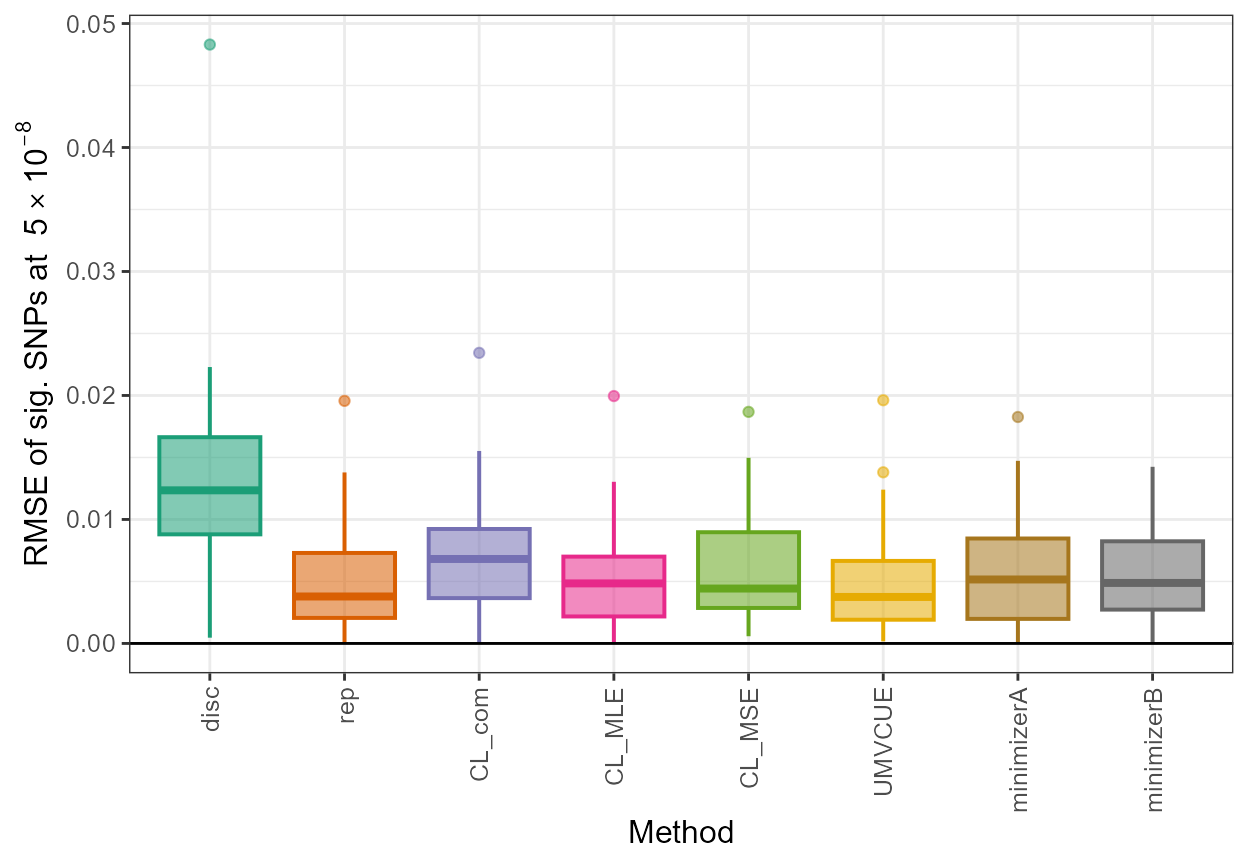
In addition, we can gain a visual insight into the adjustments made by these functions by constructing a density plot with the adjusted absolute values along with the naive estimates and the true absolute \(\beta\) values of significant SNPs, as follows:
true <- data.frame(rsid = c(out_CL$rsid), beta_disc =c(out_CL$beta_disc), se_disc =c(out_CL$se_disc),adj_beta=true_beta[out_CL$rsid],method=c(rep("true",33)))
all_resultsA <- rbind(all_results[,1:5],true)

ggplot(all_resultsA, aes(x=abs(adj_beta),colour=method,fill=method)) + geom_density(alpha=0.05,size=1) + scale_fill_manual(values=c(col[1],col[2],col[3],col[4],col[5],col[6],col[7],col[8],col1[11])) + scale_color_manual(values=c(col[1],col[2],col[3],col[4],col[5],col[6],col[7],col[8],col1[11])) + xlim(-0.01,0.08) +
  ylab("Density") + xlab(expression(paste("|", beta, "| " , "of sig. SNPs at  ", 5%*%10^-8))) + theme_bw() +  theme(text = element_text(size=12)) + labs(fill = "Method",colour="Method")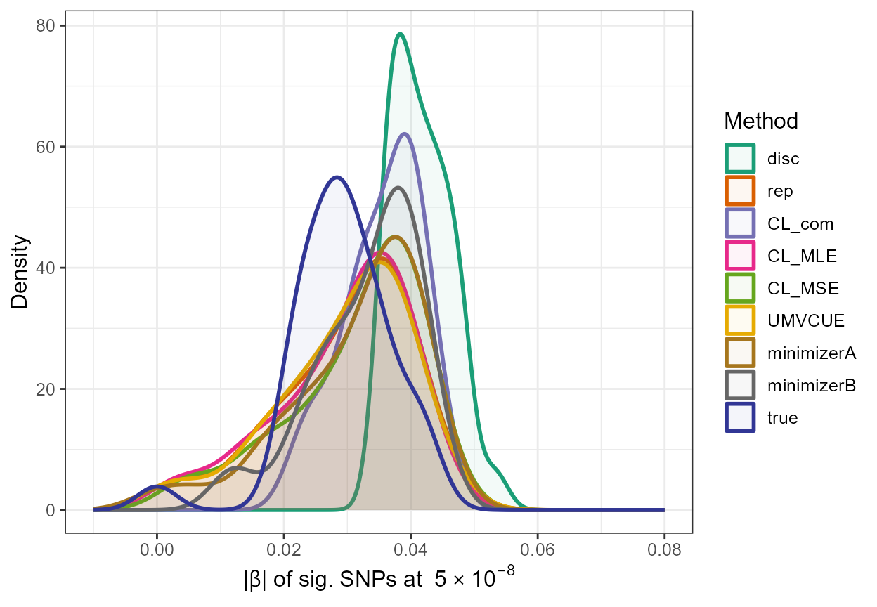
\(\star\) Note: In
the above plot, it can be seen that there must be very little difference
between the replication estimates and the adjusted estimates obtained
using the UMVCUE method as the density curves of rep and
UMVCUE can be seen to nearly overlap completely.
\(~\) \(~\)
Using empirical Bayes and bootstrap methods with replication data sets
When a replication data set is also available, as has been described
throughout this vignette, we also potentially have the option to employ
the empirical Bayes and bootstrap methods. We have seen this work well
in simulations, especially in terms of reducing the mean square error
(MSE) and thus, consider exploration of their implementation in this
setting. With data in the form described above similar to
disc_stats and rep_stats, implementation of
both methods could take place on the combined estimator as shown
below:
## combined estimator:
com_stats <- data.frame(rsid = disc_stats$rsid, beta = ((((rep_stats$se)^2)*(disc_stats$beta))+(((disc_stats$se)^2)*(rep_stats$beta)))/(((disc_stats$se)^2) + ((rep_stats$se)^2)), se = sqrt((((disc_stats$se)^2)*((rep_stats$se)^2))/(((disc_stats$se)^2) + ((rep_stats$se)^2))))
## apply methods:
out_EB_com <- empirical_bayes(com_stats)
out_boot_com <- BR_ss(com_stats,seed_opt=TRUE,seed=2020)
## rearrange data frames with SNPs ordered 1,2,3..
out_EB_com <- dplyr::arrange(out_EB_com,out_EB_com$rsid)
out_boot_com <- dplyr::arrange(out_boot_com,out_boot_com$rsid)
out_EB_com <- data.frame(rsid = disc_stats$rsid, beta_disc = disc_stats$beta, se_disc = disc_stats$se, beta_rep =rep_stats$beta, se_rep = rep_stats$se, beta_EB=out_EB_com$beta_EB)
out_boot_com <- data.frame(rsid = disc_stats$rsid, beta_disc = disc_stats$beta, se_disc = disc_stats$se, beta_rep =rep_stats$beta, se_rep = rep_stats$se, beta_boot=out_boot_com$beta_BR_ss)
## reorder data frames based on significance in discovery data set:
out_EB_com <- dplyr::arrange(out_EB_com, dplyr::desc(abs(out_EB_com$beta_disc/out_EB_com$se_disc)))
out_EB_com <- out_EB_com[abs(out_EB_com$beta_disc/out_EB_com$se_disc) > stats::qnorm((5e-8)/2, lower.tail=FALSE),]
head(out_EB_com)
#> rsid beta_disc se_disc beta_rep se_rep beta_EB
#> 1 7815 0.04771727 0.006568299 0.03581301 0.006568299 0.03941144
#> 2 3965 0.04609999 0.006346232 0.04351227 0.006346232 0.04253200
#> 3 4998 -0.04527792 0.006458823 -0.03903791 0.006458823 -0.03721732
#> 4 9917 0.04164616 0.006334188 0.04179376 0.006334188 0.03945015
#> 5 7261 0.04162686 0.006343244 0.03680436 0.006343244 0.03694256
#> 6 6510 0.04254046 0.006500057 0.03778228 0.006500057 0.03783212
out_boot_com <- dplyr::arrange(out_boot_com, dplyr::desc(abs(out_boot_com$beta_disc/out_boot_com$se_disc)))
out_boot_com <- out_boot_com[abs(out_boot_com$beta_disc/out_boot_com$se_disc) > stats::qnorm((5e-8)/2, lower.tail=FALSE),]
head(out_boot_com)
#> rsid beta_disc se_disc beta_rep se_rep beta_boot
#> 1 7815 0.04771727 0.006568299 0.03581301 0.006568299 0.03717765
#> 2 3965 0.04609999 0.006346232 0.04351227 0.006346232 0.03742383
#> 3 4998 -0.04527792 0.006458823 -0.03903791 0.006458823 -0.03634219
#> 4 9917 0.04164616 0.006334188 0.04179376 0.006334188 0.03663213
#> 5 7261 0.04162686 0.006343244 0.03680436 0.006343244 0.03512965
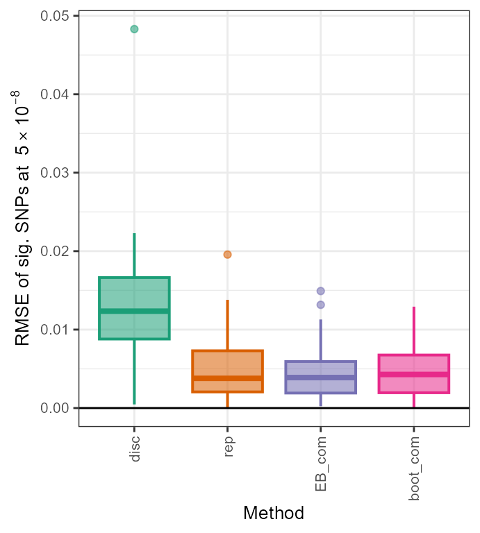
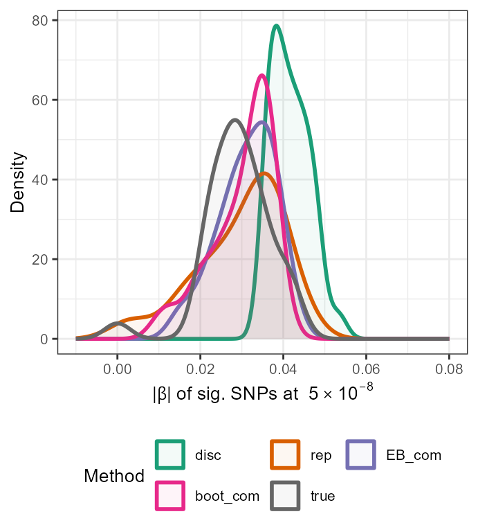
#> 6 6510 0.04254046 0.006500057 0.03778228 0.006500057 0.03598019We now compute similar evaluation metrics to above and produce the two plots in order to demonstrate the performance of the above approaches.
## rmse
rmse <- data.frame(disc = sqrt(mean((out_CL$beta_disc - true_beta[out_CL$rsid])^2)), rep = sqrt(mean((out_CL$beta_rep - true_beta[out_CL$rsid])^2)), EB_com = sqrt(mean((out_EB_com$beta_EB - true_beta[out_CL$rsid])^2)), boot_com = sqrt(mean((out_boot_com$beta_boot - true_beta[out_CL$rsid])^2)))
rmse
#>         disc         rep      EB_com    boot_com
#> 1 0.01528707 0.007126685 0.005638044 0.005754051

## bias positive
bias_up <- data.frame(disc = mean(out_CL$beta_disc[pos_sigA] - true_beta[pos_sig]), rep = mean(out_CL$beta_rep[pos_sigA] - true_beta[pos_sig]), EB_com = mean(out_EB_com$beta_EB[pos_sigA] - true_beta[pos_sig]), boot_com = mean(out_boot_com$beta_boot[pos_sigA] - true_beta[pos_sig]))
bias_up
#>         disc           rep      EB_com     boot_com
#> 1 0.01268454 -0.0005214959 0.002295151 1.917213e-05

## bias negative
bias_down <- data.frame(disc = mean(out_CL$beta_disc[neg_sigA] - true_beta[neg_sig]), rep = mean(out_CL$beta_rep[neg_sigA] - true_beta[neg_sig]), EB_com = mean(out_EB_com$beta_EB[neg_sigA] - true_beta[neg_sig]), boot_com = mean(out_boot_com$beta_boot[neg_sigA] - true_beta[neg_sig]))
bias_down
#>          disc          rep       EB_com   boot_com
#> 1 -0.01250495 -0.001461264 -0.002040202 -0.0020347
par(mfrow = c(2, 1))
all_results <- data.frame(rsid = c(rep(out_CL$rsid,4)), beta_disc = c(rep(out_CL$beta_disc,4)), se_disc = c(rep(out_CL$se_disc,4)), adj_beta = c(out_CL$beta_disc,out_CL$beta_rep,out_EB_com$beta_EB,out_boot_com$beta_boot), method = c(rep("disc",33),rep("rep",33),rep("EB_com",33),rep("boot_com",33)))
all_results$rmse <- sqrt((all_results$adj_beta - true_beta[all_results$rsid])^2)
all_results$method <- factor(all_results$method, levels=c("disc","rep","EB_com", "boot_com"))
ggplot(all_results,aes(x=method,y=rmse,fill=method, color=method)) + geom_boxplot(size=0.7,aes(fill=method, color=method, alpha=0.2)) + scale_fill_manual(values=c(col[1],col[2],col[3],col[4])) + scale_color_manual(values=c(col[1],col[2],col[3],col[4]))  + xlab("Method") +
  ylab(expression(paste("RMSE of sig. SNPs at  ", 5%*%10^-8))) + theme_bw() + geom_hline(yintercept=0, colour="black") +  theme(axis.text.x=element_text(angle=90, vjust=0.5, hjust=1),text = element_text(size=10),legend.position = "none", strip.text = element_text(face="italic"))
true <- data.frame(rsid = c(out_CL$rsid), beta_disc =c(out_CL$beta_disc), se_disc =c(out_CL$se_disc),adj_beta=true_beta[out_CL$rsid],method=c(rep("true",33)))
all_resultsA <- rbind(all_results[,1:5],true)
ggplot(all_resultsA, aes(x=abs(adj_beta),colour=method,fill=method)) + geom_density(alpha=0.05,size=1) + scale_fill_manual(values=c(col[1],col[2],col[3],col[4],col[8])) + scale_color_manual(values=c(col[1],col[2],col[3],col[4],col[8])) + xlim(-0.01,0.08) +
  ylab("Density") + xlab(expression(paste("|", beta, "| " , "of sig. SNPs at  ", 5%*%10^-8))) + theme_bw() +  theme(text = element_text(size=10),legend.position="bottom") + labs(fill = "Method",colour="Method") +guides(fill=guide_legend(nrow=2,byrow=TRUE))