This R package, winnerscurse, has been designed to provide easy access to published methods which aim to correct for Winner’s Curse, using summary statistics from genome-wide association studies (GWASs). With merely estimates of the variant-trait association, beta, and corresponding standard error, se, for each variant or single nucleotide polymorphism (SNP), this package permits users to implement adjustment methods to obtain more accurate estimates of the true association values. Methods can be applied to data relating to both quantitative and binary traits. This package contains functions which can be implemented with just the summary statistics from a discovery GWAS as well as functions which require summary data from both discovery and replication GWASs. Users can also obtain confidence intervals and standard errors for certain adjusted association estimates.
Installation
You can install the current version of winnerscurse from GitHub with:
install.packages("remotes")
remotes::install_github("amandaforde/winnerscurse")
Winner’s Curse
The Winner’s Curse is a statistical effect which generally results in the exaggeration of SNP-trait association estimates in the study that discovered these associations. To briefly explain this concept further, genome-wide association studies are used to detect genetic variants or SNPs that are associated with a trait of interest and subsequently, estimate the size of these associations. However, due to this phenomenon termed as Winner’s Curse, the association estimates of the variants that are seen to be most associated with the trait in the study tend to be upward biased and greater in magnitude than their true values.
However, Winner’s Curse isn’t just a phenomenon related to genetic association studies and thus, a better understanding of the concept may be gained through reflecting on the following simpler examples.
Firstly, let us consider the English football league, the Premier League, and suppose football players are ranked based on the number of goals scored in one season. The top ranking players, the ‘winners’, are most likely players who had an above average season, perhaps those who were at the peak of their career and fitness. However, across many seasons, these highly ranked players may not score as many goals nor be as outstanding consistently. For example, take Leicester City player, Jamie Vardy, for instance, and imagine that we wish to estimate the average number of goals he scores per Premier League season. If we only had information regarding the 2019/2020 season in which he was awarded the Premier League Golden Boot, i.e. he was the leading goalscorer in the league that season, then we would have to use the number of goals he scored that season (23) as an estimate of the average number of goals he scores per season. However, in reality, according to Premier League statistics, between 2014 and 2022, the true average number of goals scored by Jamie Vardy per season was approximately 16.6. Therefore, the estimate of 23 obtained using the single data set from 2019/2020 is clearly an overestimation of the true average number of goals scored by Jamie Vardy per season, demonstrating the Winner’s Curse concept.

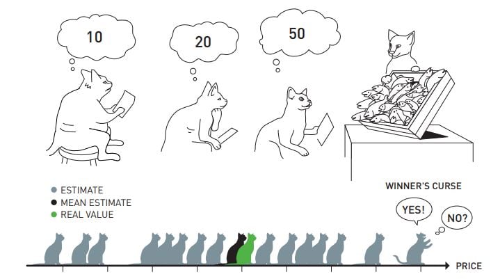
In fact, the term Winner’s Curse first arose in the realm of auction theory. Imagine a common value auction in which each potential buyer independently estimates the value of the item up for auction and submits this as their bid. The winner of the auction is then the bidder who makes the highest estimate and thus, has submitted the highest bid. If it is assumed that the average bid is close to the true value of the item, then this winner will most likely pay more for the item than its true value, giving rise to the phenomenon of Winner’s Curse. A nice illustration of this is shown in the image below where we see several cats bidding for a crate of fish. The real value of the crate is shown to be similar to the average of the estimates or bids given by the various cats. This then results in the cat with the highest bid, the winning cat, receiving the crate of fish but also paying much more than the crate’s true value. We say that this cat has then suffered from Winner’s Curse.
Now, let us reframe this idea of Winner’s Curse in the context of genetic association studies. The ‘winners’ here are SNPs whose effect sizes are stochastically higher in the discovery study than their true association values. Clearly, these raw effect estimates are therefore biased association estimates, especially for those SNPs who are ranked highly in the study, namely the most significant SNPs. In genetic studies, SNPs are often ranked according to their z-statistics or corresponding p-values, and are deemed as significant if their p-values are less than a pre-specified threshold. The most common threshold used in this instance is the genome-wide significance threshold of 5 × 10⁻⁸.
⋆ Note: The goal of the functions then in this package is to adjust the raw effect estimates, beta, rendering them less biased and more accurate. Several functions in this package can make adjustments using only the summary statistics obtained from a single discovery study.
Example
We now discuss a simple simulated data set of GWAS summary statistics, providing an alternative manner in which to comprehend the Winner’s Curse with a visual representation of the bias induced. We simulate summary statistics for a quantitative trait with a normal effect size distribution under the assumption that SNPs are independent. We assume a fixed array of 1,000,000 SNPs in which 1% have a true effect on the trait. In addition, we fix the heritability of the trait as moderate with a value of 0.4 and suppose that a total of 50,000 individuals have been sampled in the study. This is a similar toy data set to that used in the first vignette, ‘Methods for use with discovery GWAS’ and thus, a more detailed description of how the function sim_stats was used to simulate this data set can be found there.
The true effect sizes, true_beta, were first generated and then used to simulate one effect estimate, beta_hat for each SNP. This process is similar to performing a single GWAS or only having access to the goals scored by football players in one league season. In this simulation scenario, we can thus easily compare beta_hat with beta for each SNP. With real data sets, we are not as fortunate and hence, this provides motivation to establish suitable Winner’s Curse correction methods which will aim to reduce or eliminate the bias witnessed in the effect estimates of significant SNPs. The table below shows the 6 SNPs in our toy data set which have been deemed most extreme according to their z-statistic. It contains the values for beta_hat and true_beta, with the bias induced by Winner’s Curse evident. 5 of the beta_hat values are an overestimation of their corresponding true effect size.

In addition to the above table, there are a number of ways in which we can attempt to visualise the existence of Winner’s Curse in our toy data set. Firstly, in a similar manner to how we visualise results in the first vignette, we can construct a density plot of the true absolute effect sizes, |β|, along with the estimated absolute effect sizes, |β̂|, for the 34 SNPs which have been deemed significant according to the genome-wide significance threshold of 5 × 10⁻⁸. In the plot below, these effect sizes are termed as ‘true’ and ‘naive’, respectively. As expected, we witness the turquoise curve of the estimated effect, ‘naive’, lying to the right of the true effect orange curve, ‘true’. This provides a strong indication that a large number of the estimated effects of these extreme SNPs are greater than their corresponding true values.

Therefore, in visual terms, we would like the functions of our package to produce estimates which are more in line with the true values, i.e. shifted more towards the orange density plot on the left, avoiding the obvious inflation incurred by the ‘naive’ association estimates here.
Another interesting way in which this Winner’s Curse induced bias can be visualised is to plot z vs bias for the simulated data set in which z = beta_hat/se and bias = beta_hat - beta. This z vs bias plot takes the same form as those seen in S2 Fig in Forde et al. (2023). In the plot below, the bright red line corresponds to the significance threshold of 5 × 10⁻⁸ while the darker red line relates to 5 × 10⁻⁴. The points corresponding to SNPs which are significantly overestimated and are significant at a threshold of 5e-4 are coloured in grey. A SNP is defined as being significantly overestimated or as having a significantly more extreme effect size estimate, at the 2.5% significance level, if it satisfies the condition: |beta_hat| > |beta| + 1.96se. It can be seen clearly in the plot below that significant SNPs with negative z-statistics tend to also have negative bias values and vice versa for the significant SNPs with positive z-statistics, which is as expected due to Winner’s Curse.

⋆ Note: In order to appropriately use the functions in this package, GWAS summary statistics must be in the form of a data frame with three columns rsid, beta and se, in which the first column, titled rsid, contains the SNP ID number, the second column, named beta, contains the effect size estimate while the third column, se holds the corresponding estimated standard error.