Standard errors and confidence intervals of adjusted estimates
standard_errors_confidence_intervals.RmdThis third vignette briefly illustrates how our R package,
winnerscurse, can be used to generate standard
errors and confidence intervals for certain
adjusted association estimates, obtained using the ‘discovery
only’ Winner’s Curse correction methods. Here, we
demonstrate the functionality of the functions, se_adjust
and cl_interval, using a simulated data set of GWAS summary
statistics and discuss the properties of each function. We create the
same toy data set as that used in the first
vignette:
set.seed(1998)
sim_dataset <- sim_stats(nsnp=10^6,h2=0.4,prop_effect=0.01,nid=50000)
## simulated GWAS summary statistics
summary_stats <- sim_dataset$disc
Standard errors of adjusted estimates
-
The function
se_adjusthas three parameters:-
summary_data: a data frame in the form as described previously, with columnsrsid,betaandse -
method: the user is required to specify which ‘discovery only’ method they wish to implement in order to obtain standard errors;"empirical_bayes","BR_ss"or"FDR_IQT", which represent the use of the empirical Bayes method, the bootstrap method, or FDR Inverse Quantile Transformation, respectively. All three Winner’s Curse correction methods are detailed in the first vignette. -
n_boot: a numerical value which defines the number of bootstraps to be used, the default option is 100 bootstraps,n_boot=100. The function requires that this number is greater than 1.
-
se_adjustoutputs a data frame in a similar format to other functions included in this R package. It includes thebetaestimates obtained after adjustment using the specified method,method, as well as an additional columnadj_se. This column contains a value which approximates the standard error of the adjusted association estimate.se_adjustuses a parametric bootstrap approach. Firstly, using the inputted data set,n_bootindividual data sets are created as follows. For each bootstrap \(\text{b} = 1, \dots\)n_boot, a value for \(\hat\beta^{(\text{b})}\) is generated for each SNP from a normal distribution centred at the naive \(\hat\beta\) with standard error, \(\text{se}(\hat\beta)\): \[\hat\beta^{(\text{b})} \sim N(\hat\beta, \text{se}(\hat\beta)).\]The specified method,
method, is then implemented on each of then_bootdata sets and so for each SNP, we now haven_bootadjusted ‘bootstrapped’ \(\hat\beta\) estimates. The standard error is then easily obtained by applying the functionsdto this set of adjusted estimates for each SNP.It is important to note that the use of bootstrapping with large data sets can be quite computationally intensive. On a personal computer, executing 100 bootstraps can result in
se_adjusttaking between 1 and 3 minutes to provide an output with a data set such as the one described here. As expected,BR_sstends to take the longest of the three methods.An example of the implementation of this function for each of the three methods is given below. For ease of demonstration, a mere 10 bootstraps is used on all occasions. However, a value of
n_bootas small as this is not advised in practice.
out_EB <- se_adjust(summary_data = summary_stats, method = "empirical_bayes", n_boot=10)
head(out_EB)
#>   rsid        beta          se     beta_EB      adj_se
#> 1 7815  0.04771727 0.006568299  0.04599530 0.008669139
#> 2 3965  0.04609999 0.006346232  0.04443623 0.008500261
#> 3 4998 -0.04527792 0.006458823 -0.03999539 0.010010348
#> 4 9917  0.04164616 0.006334188  0.03998556 0.004601265
#> 5 7261  0.04162686 0.006343244  0.03996389 0.008016920
#> 6 6510  0.04254046 0.006500057  0.04083638 0.009074620

out_BR_ss <- se_adjust(summary_data = summary_stats, method = "BR_ss", n_boot=10)
head(out_BR_ss)
#>   rsid        beta          se  beta_BR_ss      adj_se
#> 1 7815  0.04771727 0.006568299  0.03499261 0.006790539
#> 2 3965  0.04609999 0.006346232  0.03380467 0.006879619
#> 3 4998 -0.04527792 0.006458823 -0.03203960 0.002972599
#> 4 9917  0.04164616 0.006334188  0.02836485 0.004280097
#> 5 7261  0.04162686 0.006343244  0.02830782 0.004225297
#> 6 6510  0.04254046 0.006500057  0.02886472 0.004706941

out_FIQT <- se_adjust(summary_data = summary_stats, method = "FDR_IQT", n_boot=10)
head(out_FIQT)
#>   rsid        beta          se   beta_FIQT      adj_se
#> 1 7815  0.04771727 0.006568299  0.03422825 0.009403474
#> 2 3965  0.04609999 0.006346232  0.03307103 0.007694662
#> 3 4998 -0.04527792 0.006458823 -0.03188772 0.009541773
#> 4 9917  0.04164616 0.006334188  0.02823824 0.007188336
#> 5 7261  0.04162686 0.006343244  0.02827861 0.006387643
#> 6 6510  0.04254046 0.006500057  0.02897770 0.004577303
\(\star\) Note: Due to the nature of the conditional likelihood methods, i.e. adjustments are only made to association estimates of SNPs with \(p\)-values less than a chosen significance threshold, it is not possible to obtain standard errors of the conditional likelihood adjusted association estimates in the above manner.
\(\star\) Note:
Currently, this package does not provide a way to create confidence
intervals for adjusted association estimates obtained using the three
methods mentioned above, empirical Bayes, FDR Inverse Quantile
Transformation and bootstrap. However, one option that could be
considered is to take an approach similar to that of
se_adjust and obtain quantiles by means of parametric
bootstrap. Unfortunately, in order to ensure accurate quantiles, this
would require many n_boot simulated data sets to which the
correction method of choice is applied, resulting in a very
computationally intensive process. For this reason, a function that
would generate suitable quantiles for each adjusted association estimate
has been omitted from the R package for now.
Confidence intervals for estimates adjusted by conditional likelihood methods
The function
cl_intervalimplements the conditional likelihood methods described in Ghosh et al. (2008) for each significant SNP and together with the three adjusted estimates, provides a single confidence interval for each SNP. As well as a data set in the form of a data frame with columnsrsid,betaandse,cl_intervalrequiresalpha, a value which specifies the significance threshold andconf, a value between 0 and 1 which determines the confidence interval. The default setting forconfis 0.95.This confidence interval for the adjusted estimate is specified in Ghosh et al. (2008). With \(\mu = \frac{\beta}{\text{se}(\beta)}\) and \(z = \frac{\hat\beta}{\hat{\text{se}(\hat\beta)}}\), consider the acceptance region \(A(\mu,1-\eta)\), which is defined as the interval between the \(\eta/2\) and \(1-\eta/2\) quantiles of the conditional density, \(p_{\mu}(z | \mid Z \mid > c )\). Having obtained the lower and upper boundaries of this acceptance region, the desired confidence interval is given as: \[(\mu_{\text{lower}}\hat{\text{se}(\hat\beta)}, \mu_{\text{upper}}\hat{\text{se}(\hat\beta)}).\]
In the output of
cl_interval, thelowercolumn holds the values of the lower confidence limit for each SNP while theuppercolumn contains the upper confidence limit.If no SNPs are detected as significant, the function returns a warning message:
WARNING: There are no significant SNPs at this threshold.cl_intervalcan be used in conjunction with the toy data set as shown below, in whichalphais specified as5e-8and a 95% confidence interval is desired:
out <- cl_interval(summary_data=summary_stats, alpha = 5e-8, conf_level=0.95)
head(out)
#>   rsid        beta          se    beta.cl1    beta.cl2    beta.cl3       lower
#> 1 7815  0.04771727 0.006568299  0.04709173  0.04575084  0.04642129  0.02855506
#> 2 3965  0.04609999 0.006346232  0.04549476  0.04419814  0.04484645  0.02758022
#> 3 4998 -0.04527792 0.006458823 -0.04421716 -0.04238468 -0.04330092 -0.05716545
#> 4 9917  0.04164616 0.006334188  0.03909824  0.03598923  0.03754373  0.01349641
#> 5 7261  0.04162686 0.006343244  0.03900942  0.03584977  0.03742959  0.01319315
#> 6 6510  0.04254046 0.006500057  0.03975867  0.03645266  0.03810567  0.01304579
#>         upper
#> 1  0.06008004
#> 2  0.05804426
#> 3 -0.02376903
#> 4  0.05248926
#> 5  0.05245207
#> 6  0.05358307
\(\star\) Note:
Similar to condlike_rep discussed in the second
vignette, cl_interval also uses the R function
uniroot which generates values for upper and
lower numerically and thus, we advise users to be cautious
of uniroot’s possible failure to obtain appropriate values
in certain circumstances. In practice, this failure has been witnessed
to occur very rarely. However, in order to ensure a greater possibility
that cl_interval will produce appropriate confidence
intervals for each significant SNPs, cl_interval can only
be used with data sets in which the absolute value of the
largest naive \(z\)-statistic
is less than 150.
In the final part of this vignette, we will evaluate and visualise the above obtained confidence intervals. Firstly, we will consider computing the coverage of these confidence intervals for the significant SNPs, i.e. we calculate what percentage of these confidence intervals contain the true association estimate, as shown below.
## Simulated true effect sizes:
true_beta <- sim_dataset$true$true_beta[out$rsid]

## coverage
coverage <- (sum((true_beta > out$lower) & (true_beta < out$upper))/length(true_beta))*100
coverage
#> [1] 96.9697
Next, we construct a simple forest plot to illustrate the
adjusted association estimates and corresponding confidence intervals
for each SNP in our simulated data set. Of the three conditional
likelihood adjusted estimates, we include beta.cl2 as the
effect size in our plot.
library(ggplot2)
library(RColorBrewer)
col <- brewer.pal(8,"Dark2")
out$index <- c(33:1)
out$pos <- out$beta > 0
ggplot(data=out, aes(y=index, x=beta.cl2, xmin=lower, xmax=upper, color=pos)) +
  geom_point() +
  geom_errorbarh(height=.5) +
  scale_color_manual(values=c(col[1],col[2])) +
scale_y_continuous(name = "SNP ID", breaks=1:nrow(out), labels=out$rsid) + xlab(expression(paste("Effect size of sig. SNPs at ", 5%*%10^-8))) + theme_bw() + geom_vline(xintercept=0, colour="black",linetype='dashed', alpha=.5) + theme(text = element_text(size=10),legend.position="none") 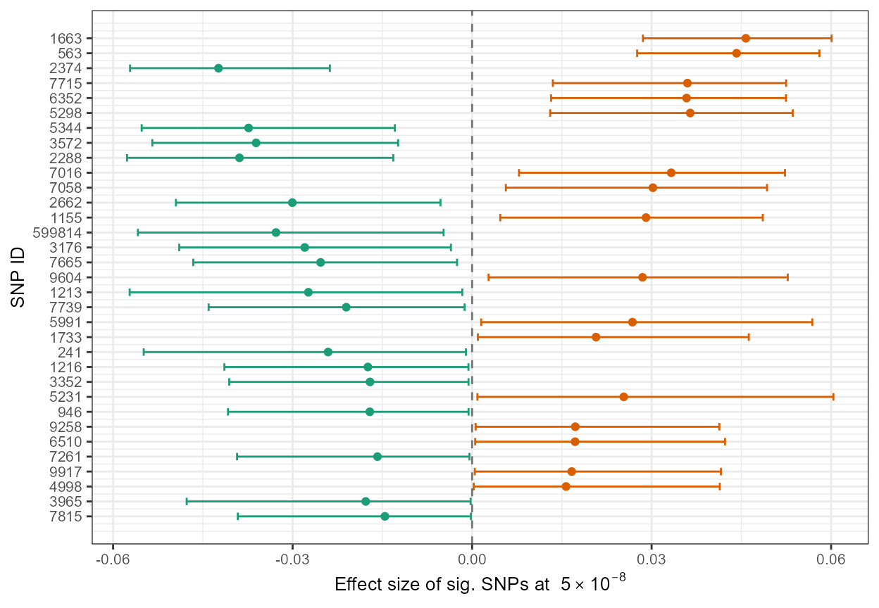
\(~\) \(~\)